settings
say we have model that $Y = \beta * X + e$, where $e$ follows a normal distribution (with mean 0, and an unknown variance $\sigma$). X, Y represent genotypes (0, 1, 2, binomial distribution), phenotypes ($-\inf, +\inf$), respectively.
Let n for sample size of X and Y, the task is to estimate $\beta$ based on observations.
MLE and its Confidence Intervals ($CI_{MLE}$)
Since $e$ follows a normal distribution, treat X as constant in regression, $Y_{i}$ follows a normal distribution with $N(\beta * X_{i}, \sigma^2)$.
We have: $$ \mathbf{L}(Y|X, \beta, \sigma) = \prod \mathbf{L}(y_{i}|x_{i}, \beta, \sigma) $$
$$ = (\frac{1}{\sqrt{2\pi}\sigma})^n \exp (\sum-\frac{(y_{i}-\beta x_{i})^2}{2 \sigma^2}) $$ $$ \ln \mathbf{L} = -\frac{n}{2} \ln 2\pi - n\ln\sigma + \sum-\frac{(y_{i}-\beta x_{i})^2}{2\sigma^2} $$
$$ \partial \ln \mathbf{L} / \partial \beta = \sum y_{i}x_{i} / \sigma^2 - \sum\beta x_{i}^2 / \sigma^2 $$
let $$ 0 = \sum y_{i}x_{i} - \sum\hat\beta_{MLE} x_{i}^2 $$ we have $\hat\beta_{MLE} = \frac {\sum y_{i}x_{i}}{\sum x_{i}^2}$.
we can then establish its $CI_{MLE}$ around its pivotal quantity. The critical value $t_{0.025}$ depends on the df hence the shape of T. Thus,
$$ (\hat\beta_{MLE} - \beta) / SE (\hat\beta_{MLE}) \sim T(df=n-1) $$
$$ -t_{0.025} < (\hat\beta_{MLE} - \beta) / SE (\hat\beta_{MLE}) < t_{0.025} $$
The CI $$ (\hat\beta_{MLE}-t_{0.025} SE (\hat\beta_{MLE}), \hat\beta_{MLE}+ t_{0.025} SE (\hat\beta_{MLE})) $$
Bayesian Credible Intervals ($CI_{B}$)
For simplification from marginal posterior distribution, we treat true variance of the error $\sigma$ as known here. We assume the $\beta$ has a priori std normal distribution.
$$ \mathbf{P}^\ast(\beta|y_{1},…,y_{n}) \propto \mathbf{L}(y_{1},…,y_{n}|\beta) \cdot \mathbf{P}(\beta) $$
$$ … \propto \frac{1}{\sqrt{2\pi}} \cdot \exp (-\frac{\beta^2}{2})\cdot (\frac{1}{\sqrt{2\pi}\sigma})^n \cdot \exp (\sum (- \frac {(y_{i}-\beta x_{i})^2}{2\sigma^2}) $$ $$ … \propto \exp [-1/2(\beta^2 - \sum \frac {-y_{i}^2 +2 \beta x_{i} y_{i} - \beta^2 x_{i}^2}{\sigma^2})] $$
$$ … \propto \exp [-1/2 (\beta^2(1+ \sum \frac {x_{i}^2}{\sigma^2}) - 2\beta \sum \frac {x_{i} y_{i}}{\sigma^2} + \sum \frac{y_{i}^2}{\sigma^2})] $$
Since the product of normal distributions is guaranteed to be normal, to match the form of normal distribution, we have posterior distribution of $\beta$ with: $$ \frac{1}{\sigma_{p}^2} = 1 + \frac{\sum x_{i}^2}{\sigma^2} $$ $$ \mu_{p} = \sigma_{p}^2 (\frac {\sum x_{i}y_{i}}{\sigma^2}) [eq.1] $$
And the $\hat \beta_{B} = \mu_{p}$. For any normally distributed random variable, we can standardise it to a Z distribution. We know critical value $z_{0.025}=1.96$, thus for a 95 CI: $$-1.96 < (\beta - \mu_{p})/\sigma_{p} < 1.96 $$
So , $(\mu_{p} - 1.96\sigma_{p},\mu_{p} + 1.96\sigma_{p})$.
Note that, the Bayes estimator $\hat \beta_{B}$ is a weighted $\hat\beta_{MLE}$: $\hat \beta_{B} = \frac{\sum x_{i} y_{i}}{\sigma^2+ \sum x_{i}^2} = \frac{\sum x_{i}^2}{\sigma^2+ \sum x_{i}^2} * \frac {\sum y_{i}x_{i}}{\sum x_{i}^2} = \frac{\sum x_{i}^2}{\sigma^2+ \sum x_{i}^2} * \hat\beta_{MLE}$ So, with noisier data, they are further away from each other.
simulation and estimates, CI comparison
Let sample size {5, 50, 500} and variance {0.5, 15}, simulate 50 for each combination by:
_true_beta = 1.5
import numpy as np

# pick n, v in {5, 50, 500} and {0.5, 15}
genotypes = np.random.randint(0, 3, size=n).astype(float)

environmental_noise = np.random.normal(0, np.sqrt(v), size=n)

simulations = genotypes * _true_beta + environmental_noise
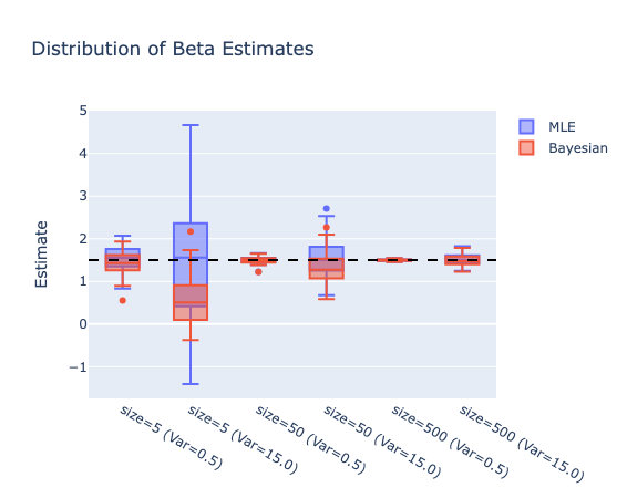
We see here that under small sample size and large variance, Bayesian estimates show a tendency to shrink toward the prior mean of 0. Two distributions converge as sample size increasing.
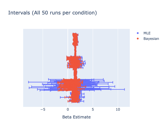 For intervals, the Credible Intervals shown stable not surprisingly we set the true variance known to Bayesian. And as indicated in eq.1, the priori works as a constraint.
A more fair comparison: treating true variance unknown for Bayesian inference
Before that we’ve treated true variance as known for simplicity. We could relax that setting by assigning the Inverse Gamma distribution to $\sigma$. The posterior distribution of $\beta$ will turn into a t-distribution. We’ll build this up in next post.
© 2026 Mike Lang. Licensed under CC BY-NC-ND 4.0. Cite as: Yapeng Mike Lang, “Relation between intervals and sample size, variance”, yplang-blog